\( \newcommand{\ket}[1]{\vert#1\rangle} \newcommand{\bra}[1]{\langle#1\vert} \newcommand{\bigket}[1]{\bigl\vert#1\bigr\rangle} \newcommand{\bigbra}[1]{\bigl\langle#1\bigr\vert} \newcommand{\class}[1]{\mathrm{#1}} \newcommand{\problem}[1]{\mathrm{#1}} \renewcommand{\natural}{\mathbb{N}} \newcommand{\real}{\mathbb{R}} \newcommand{\complex}{\mathbb{C}} \newcommand{\ip}[2]{\left\langle#1, #2 \right\rangle} \newcommand{\Tr}{\mathop{\mathrm{Tr}}\nolimits} \newcommand{\tr}{\mathop{\mathrm{tr}}\nolimits} \newcommand{\abs}[1]{\left\lvert#1 \right\rvert} \newcommand{\norm}[1]{\left\lVert#1 \right\rVert} \newcommand{\floor}[1]{\left\lfloor#1 \right\rfloor} \newcommand{\X}{\mathcal{X}} \newcommand{\Y}{\mathcal{Y}} \newcommand{\A}{\mathcal{A}} \newcommand{\B}{\mathcal{B}} \newcommand{\E}{\mathop{\mathbb{E}}} \newcommand{\Var}{\mathop{\mathrm{Var}}} \newcommand{\dif}{\mathrm{d}} \newcommand{\eps}{\epsilon} \newcommand{\sign}{\mathrm{sign}} \newcommand{\poly}{\mathrm{poly}} \newcommand{\polylog}{\mathrm{polylog}} \newcommand{\negl}{\mathrm{negl}} \newcommand{\church}[1]{\overline{#1}} \newcommand{\defeq}{\stackrel{\text{def}}{=}} \newcommand{\pair}[2]{\langle#1, #2\rangle} \newcommand{\tuple}[1]{\langle#1\rangle} \newcommand{\red}{\rightarrow} \newcommand{\reds}{\twoheadrightarrow} \newcommand{\betared}{\rightarrow_{\beta}} \newcommand{\betareds}{\twoheadrightarrow_{\beta}} \newcommand{\betaeq}{=_{\beta}} \newcommand{\betaetared}{\rightarrow_{\beta\eta}} \newcommand{\betaetareds}{\twoheadrightarrow_{\beta\eta}} \newcommand{\parared}{\rightarrow_{\|}} \newcommand{\parareds}{\twoheadrightarrow_{\|}} \newcommand{\desc}[1]{\langle#1 \rangle} \newcommand{\adv}{\mathcal{A}} \newcommand{\dis}{\mathcal{D}} \newcommand{\labelsty}[1]{\mathrm{#1}} \newcommand{\Enc}{\labelsty{Enc}} \newcommand{\Dec}{\labelsty{Dec}} \newcommand{\plain}{\labelsty{p}} \newcommand{\cipher}{\labelsty{c}} \newcommand{\PRG}{\labelsty{PRG}} \newcommand{\Commit}{\labelsty{Com}} \newcommand{\oracle}{\mathcal{O}} \newcommand{\Sim}{\labelsty{Sim}} \newcommand{\comp}{\labelsty{c}} \newcommand{\view}{\labelsty{view}} \newcommand\TIME{\class{TIME}} \newcommand\SPACE{\class{SPACE}} \newcommand\SIZE{\class{SIZE}} \newcommand\NTIME{\class{NTIME}} \newcommand\NSPACE{\class{NSPACE}} \newcommand\BQP{\class{BQP}} \newcommand\BPP{\class{BPP}} \newcommand\QMA{\class{QMA}} \renewcommand\P{\class{P}} \newcommand\Ppoly{\class{P{/}poly}} \newcommand\NP{\class{NP}} \newcommand\NPC{\class{NP}\text{-complete}} \newcommand\coNP{\class{coNP}} \newcommand\MA{\class{MA}} \newcommand\AM{\class{AM}} \newcommand\QCMA{\class{QCMA}} \newcommand\EXP{\class{EXP}} \newcommand\NEXP{\class{NEXP}} \newcommand\PP{\class{PP}} \newcommand\GapP{\class{GapP}} \newcommand\IP{\class{IP}} \newcommand\QIP{\class{QIP}} \newcommand\PSPACE{\class{PSPACE}} \newcommand\NPSPACE{\class{NPSPACE}} \newcommand\MIP{\class{MIP}} \newcommand\RE{\class{RE}} \newcommand\QMAM{\class{QMAM}} \newcommand\PH{\class{PH}} \renewcommand\L{\class{L}} \newcommand\NL{\class{NL}} \newcommand\coNL{\class{coNL}} \newcommand\NLC{\class{NL}\text{-complete}} \newcommand\PPAD{\class{PPAD}} \newcommand\SharpP{\#\class{P}} \newcommand\HVPZK{\class{HVPZK}} \newcommand\HVSZK{\class{HVSZK}} \newcommand\PZK{\class{PZK}} \newcommand\SZK{\class{SZK}} \newcommand\CZK{\class{CZK}} \newcommand\val{\mathrm{val}} \newcommand\vale{\mathrm{val}^*} \newcommand\perm{\mathop{\mathrm{perm}}\nolimits} \newcommand\pathfunc{\mathrm{path}} \newcommand\SELF{\problem{SELF}} \newcommand\HALT{\problem{HALT}} \newcommand\MINTM{\problem{MIN}_\text{TM}} \newcommand\ACCTM{\problem{ACC}_\text{TM}} \newcommand\TQBF{\problem{TQBF}} \newcommand\PAL{\problem{PAL}} \newcommand\PATH{\problem{PATH}} \newcommand\LONGPATH{\problem{LONGEST\text{-}PATH}} \newcommand\SHORTPATH{\problem{SHORTEST\text{-}PATH}} \newcommand\HAMPATH{\problem{HAM\text{-}PATH}} \newcommand\HAMCYCLE{\problem{HAM\text{-}CYCLE}} \newcommand\INDSET{\problem{IND\text{-}SET}} \newcommand\MINCUT{\problem{MIN\text{-}CUT}} \newcommand\MAXFLOW{\problem{MAX\text{-}FLOW}} \newcommand\MAXCUT{\problem{MAX\text{-}CUT}} \newcommand\MAXCUTAPP{\problem{MAX\text{-}CUT\text{-}APPROX}} \newcommand\SAT{\problem{SAT}} \newcommand\PERM{\problem{PERMANENT}} \newcommand\THREESAT{3\text{-}\problem{SAT}} \newcommand\TWOSAT{2\text{-}\problem{SAT}} \newcommand\TWOUNSAT{2\text{-}\problem{UNSAT}} \newcommand\NAESAT{\problem{NAESAT}} \newcommand\REACHABILITY{\problem{REACHABILITY}} \newcommand\THREECOL{3\text{-}\problem{COLORING}} \newcommand\CLIQUE{\problem{CLIQUE}} \newcommand\COL{\problem{COLORING}} \newcommand\COMPOSITE{\problem{COMPOSITE}} \newcommand\PRIME{\problem{PRIME}} \newcommand\TSP{\problem{TSP}} \newcommand\VC{\problem{VERTEX\text{-}COVER}} \newcommand\FACTOR{\problem{FACTOR}} \newcommand\GI{\problem{GRAPH\text{-}ISO}} \newcommand\GNI{\problem{GRAPH\text{-}NONISO}} \newcommand\SHORTPROOF{\problem{SHORT\text{-}PROOF}} \newcommand\UHALT{\problem{UNARY\text{-}HALT}} \newcommand\GG{\problem{GENERAL\text{-}GEOGRAPHY}} \newcommand\FG{\problem{FORMULA\text{-}GAME}} \)

Gate Scheduling for Syndrome Measurements

Kai Zhang

1 Background

Syndrome measurements are quantum operations that detect errors by measuring the observable defined by the stabilizer generators of a quantum error-correcting code. These measurements are typically realized through circuits composed of CNOT and Hadamard gates, utilizing ancillary qubits. This project focuses on designing shallow-depth circuits capable of performing all necessary syndrome measurements efficiently.

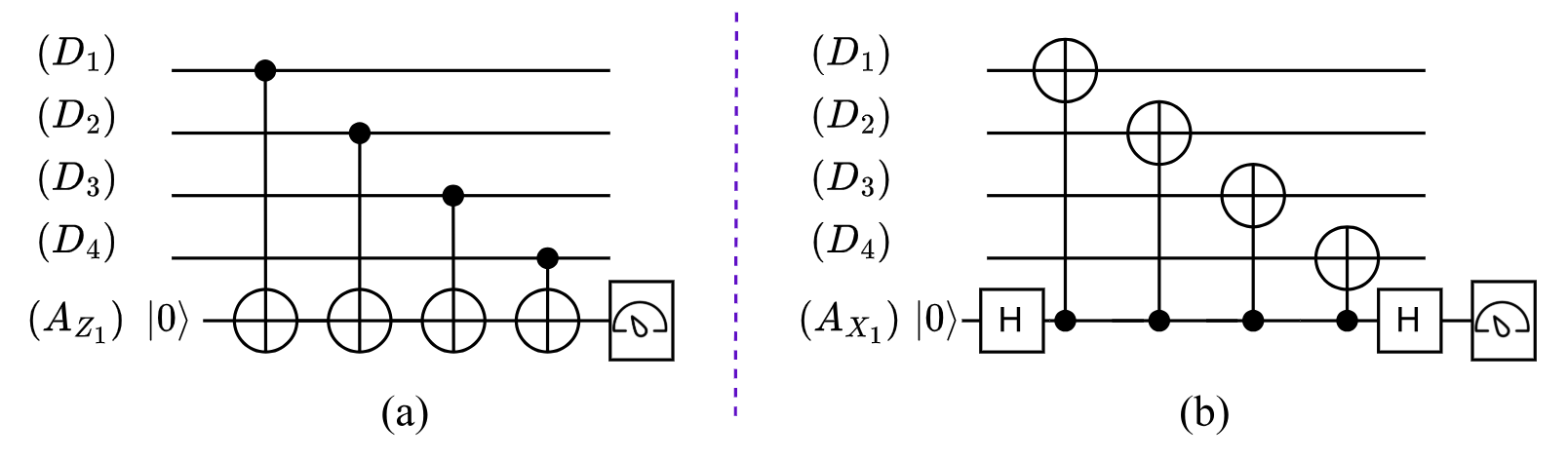
For example, in the Steane code, the syndrome measurements involve the operators \(Z_1 Z_2 Z_3 Z_4\) and \(X_1 X_2 X_3 X_4\). The corresponding circuits are shown in the following figure.

Two syndrome measurements for Steane code

Since both measurements act on qubits 1, 2, 3, and 4, and we need to measure all these two measurements (and others), gate collisions may occur if the operations are not properly scheduled.

Now we define the cost of a gate scheduling for a syndrome measurement circuit more formally, following the basic rules:

  1. For simplicity, we exclude single-qubit gates (primarily H gates) and measurements from our analysis, as done in prior work [TBLC22].

  2. We discretize time into steps (TICKs), where each CNOT gate operation consumes exactly one time unit.

  3. Parallel execution is permitted for non-conflicting CNOT gates, with the constraint that each qubit can participate in at most one CNOT operation per time step.

2 Problems

  1. Optimal Gate Scheduling: Determine the minimum-depth circuit schedule for syndrome measurement in QLDPC codes [BE21] under idealized hardware conditions (no topological constraints). You may use SMT solvers for this task.

  2. Hardware-Aware Scheduling (Research-level): Extend this to realistic hardware with limited qubit connectivity. While the problem was considered in [YZF+25] for superconducting architectures (e.g., Google’s Sycamore) with the help of SWAP gates, we instead focus on the Reconfigurable Atom Array (RAA) platform for which there are custom-made compilers (OLSQ-RAA) [TBLC22]. The challenge lies in co-optimizing syndrome measurement circuits with RAA’s reconfigurable connectivity.

3 Contacts

Kai Zhang zhang-k23@mails.tsinghua.edu.cn

Jianxin Chen chenjianxin@tsinghua.edu.cn

4 References

[YZF+25] Keyi Yin, Hezi Zhang, Xiang Fang, Yunong Shi, Travis S Humble, Ang Li, and Yufei Ding. QECC-synth: A layout synthesizer for quantum error correction codes on sparse architectures. ASPLOS 2025.

[TBLC22] Bochen Tan, Dolev Bluvstein, Mikhail D Lukin, and Jason Cong. Qubit mapping for reconfigurable atom arrays. ICCAD 2022.

[BE21] Nikolas P Breuckmann and Jens Niklas Eberhardt. Quantum low-density parity-check codes. PRX Quantum, 2(4):040101, 2021.