Seminars on Quantum Computing is a quantum computing course
designed for undergraduate students in the computer
science.
This is an incomplete set of notes prepared by Zhengfeng Ji for the
course.
Quantum Computing
What is quantum computing, or more generally, what is quantum
information science?
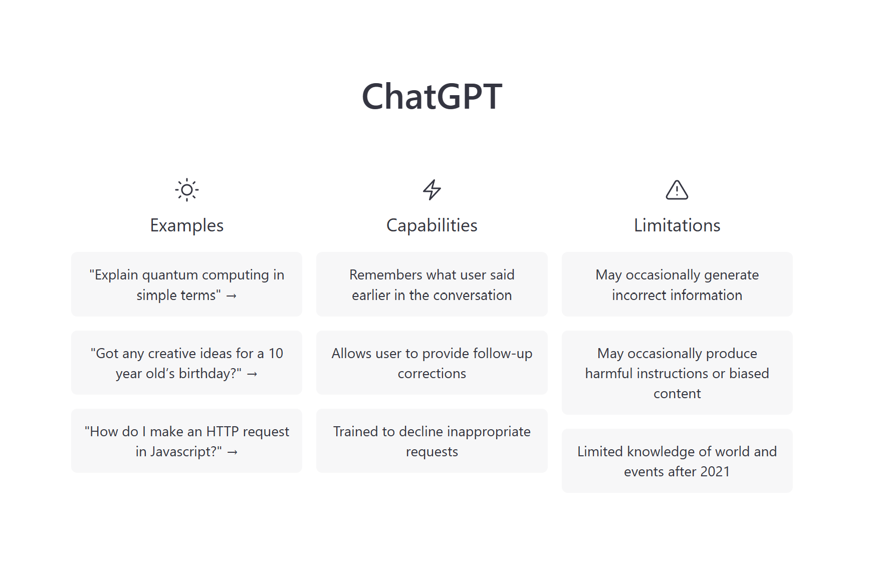
The first example question in ChatGPT: Explain quantum computing
in simple terms.
ChatGPT example questions
The answer I got was:
Quantum computing is a type of computing that uses the principles
of quantum mechanics, the science of the very small,
to process information. Instead of using classical bits, which can be
either 0 or 1, quantum computers use quantum bits or qubits, which can
be in multiple states at the same time.
This ability to exist in multiple states simultaneously is called
superposition and allows quantum computers to perform
certain calculations much faster than classical
computers. In addition, quantum computers can also use a phenomenon
called entanglement, where the state of one qubit is
correlated with the state of another, to further enhance their
computational power.
Quantum computing has the potential to solve some of the world's
most challenging problems in fields such as cryptography, drug
discovery, and climate modeling. However, building a fully functional
quantum computer remains a major scientific and engineering
challenge, and many of the applications of quantum computing are
still in the experimental stage.
You can try DeepSeek V3 and you will get something similar or
better.
They all describe the outline and motivation of this course
well!
Quantum + Information: The second quantum revolution
The success of quantum mechanics. Laser, GPS, etc.
From passive understanding of the collective effects to active
manipulation of individual particles.
History, Highlights,
Current Status
History and highlights
a. Early history: Feynman 1982, Deutsch 1985, Deutsch-Jozsa 1992 b.
Shor's factoring algorithm 1994 (breaks RSA) c. Quantum cryptography
(QKD, Bennett Brassard 84) d. Quantum teleportation (Bennett et al.,
1993) e. Simulation of quantum systems (Feynman's dream)
Current status
Primitive quantum computers are being built. Many players are
racing to build quantum computers: Google, IBM,
China, …
Different labs/companies are betting on different hardware routes:
Superconducting qubits, ion traps, photonic systems, topological
qubits, and more recently, neutral atom platforms.
Nowadays, there are programmable quantum computers with 50-1000
qubits.
Major problem: devices are noisy! The noise level
is around \(10^{-3}\).
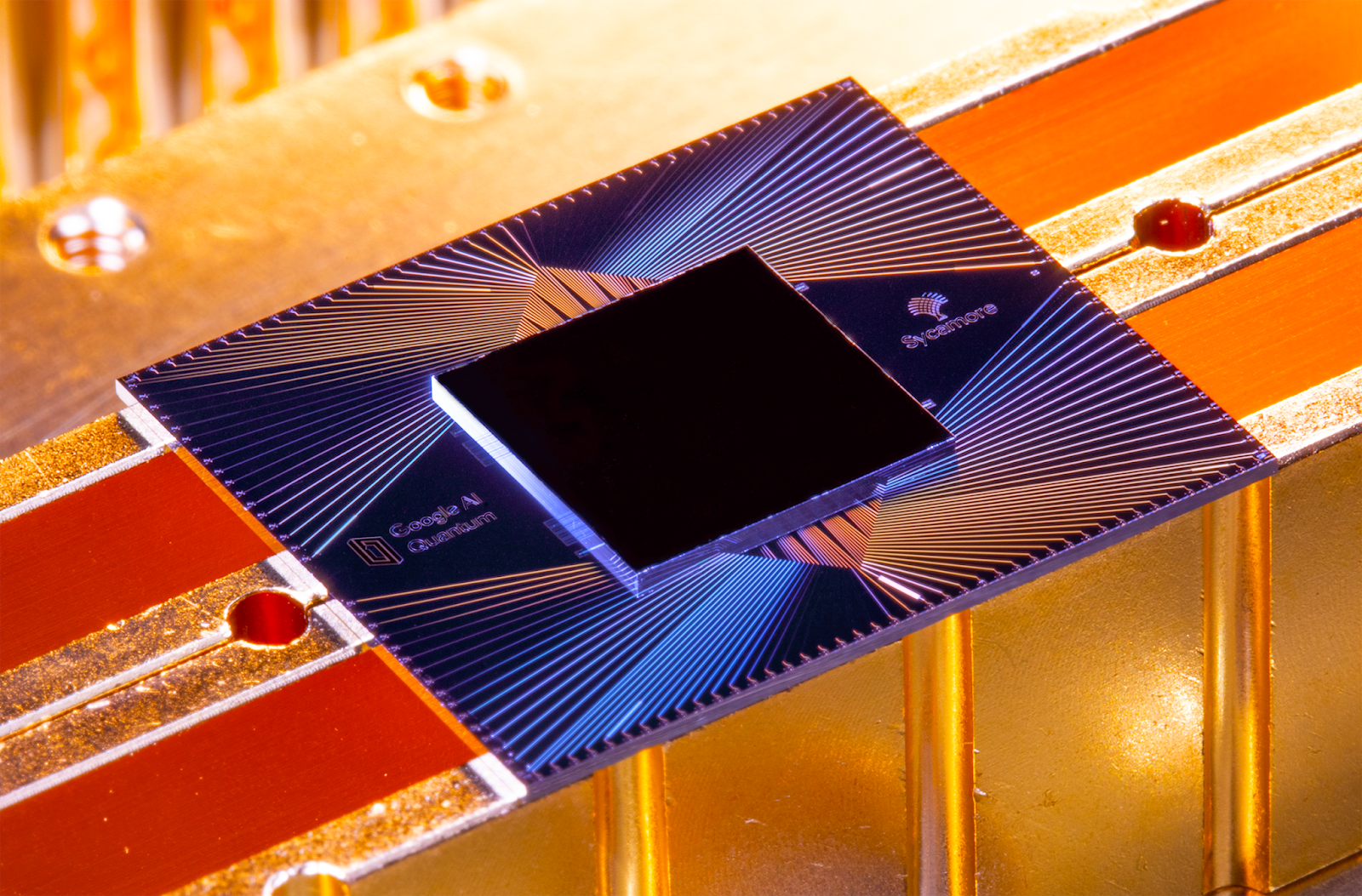
Supremacy and simulation of Google and USTC
Google Sycamore
Sycamore, 53 qubits
Zhuchongzhi, 66 qubits
The biggest competitor to quantum computers are clever classical
algorithms: In Nov 2021, a group from Chinese Academy of Sciences used
tensor network algorithms to reproduce the statistics of the Google
supremacy experiment using 512 GPUs in 15 hours.
Both Google and USTC have upgraded the system to battle against
better classical simulation methods and hardware.
On the theory side: new algorithms, new protocols,
fault-tolerant quantum computing, new insights on the power of quantum
computers
More computer scientists get involved
Hype?
a. TIME's
new cover: Quantum computers will transform our world—and create a
21st century "space race"
Quantum computing startups are all the rage, but it's unclear if
they'll be able to produce anything of use in the near
future.
Learning Quantum Computing
What you will learn in this subject
Quantum information basics (for about 1/3 of the time)
Topics in quantum computing
Research skills. Get an idea of what the big questions are for
quantum computing.
Is quantum computing hard to learn?
The mathematics is easy, the physics is hard.
There is a simple mathematical framework describing quantum
mechanics with merely four postulates, about state space, evolution,
measurement, and joint system, respectively, in both the pure state
and mixed state settings.
The postulates are simple, but the truly amazing thing to note is
how far these four simple postulates can bring us.
"Shut up and calculate!"
Reiterate over the four postulates from different
perspectives.
Lecturers
Zhengfeng Ji, Yuan Feng, and Jianxin Chen
Office: 1-707, Ziqiang S&T Building
Research direction of Zhengfeng
Quantum computing, theory of computing.
Research direction of Yuan
Quantum computing, theory of programming, mathematical
logic.
Work on projects in groups and take an idea to the extreme
(Given projects, or projects of your choice approved by your
lecturers), write an essay, present your findings.
We will grade your project by its writing and format (10%),
originality (20%), completion (10%), and presentation (20%).
Extra rule: If your project yields results deemed
near-publishable by the teachers' evaluation, you will automatically
receive an A+.
Things can only propagate through the universe at a certain
speed.
In physics, locality naturally emerges from Einstein's special
theory of relativity, which implies that no signal can propagate
faster than the speed of light.
Local Realism
Things have predetermined value, which depends on parameters in a
local region.
Einstein: I like to think the moon is there even if I am not
looking at it.
Church-Turing thesis
What is Church-Turing thesis?
TCS is mathematics but the Church-Turing thesis connects it
to physics.
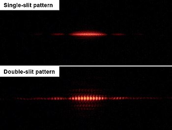
Double-slit with an observer: which path did the electron take?
If there is a conscious observer, the distribution goes back to
classical! That is the same as decoherence in a
quantum system interacting with an environment!
Quantum mechanics is an (unusual) theory using probability.
A cat isn't found in a superposition of alive and dead states,
because it interacts constantly with its environment. These
interactions essentially leak information about the 'cat system'
out.
This explains the difficulty of building a quantum computer.
Quantum computers need to be isolated well from the environment yet
still easy to manipulate.
Shor's factoring algorithm can be thought of as a large-scale
interference experiment.
Born's rule
Probability stays but monotonicity goes.
God does play dice, and an unusual one.
Einstein liked inventing phrases such as "God does not play dice,"
"The Lord is subtle but not malicious." On one occasion Bohr answered,
"Einstein, stop telling God what to do."
Instead of probabilities, quantum mechanics uses
amplitudes.
\(p = \abs{\alpha}^2\).
Let \(\alpha_i\) be the
amplitude that it lands on a position through slit \(i\).
\(\alpha=\alpha_1 +
\alpha_2\).
Example \(\alpha_1 = 1/2\) and
\(\alpha_2 = -1/2\). What is the
probability \(p\)?
Cancellation!
Linear Algebra Formulation
Linear Algebra for
Probabilities
Consider the problem of flipping a coin.
\(\Pr(\text{heads}) = p,
\Pr(\text{tails}) = q\).
Apply a transform \(X\).
In general, the transform is a matrix of transition probabilities
\(p(a|b)\).
Markov chain and stochastic matrix.
Now consider two independent coins. This leads to
the tensor product very naturally.
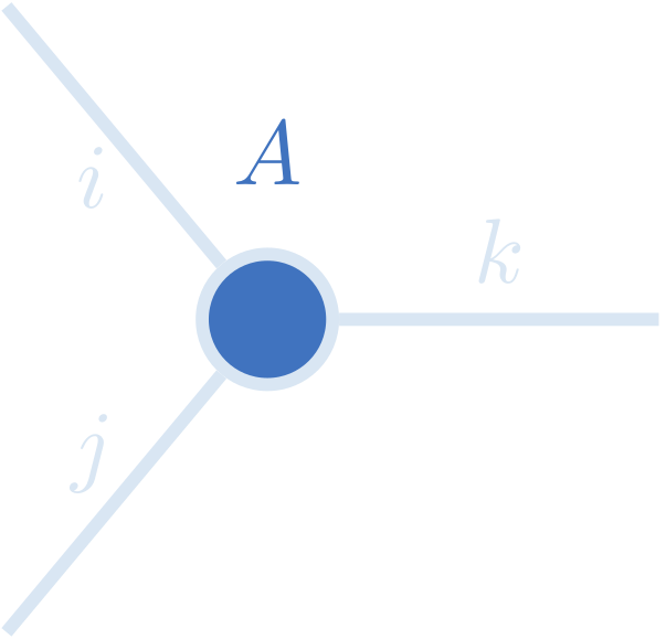
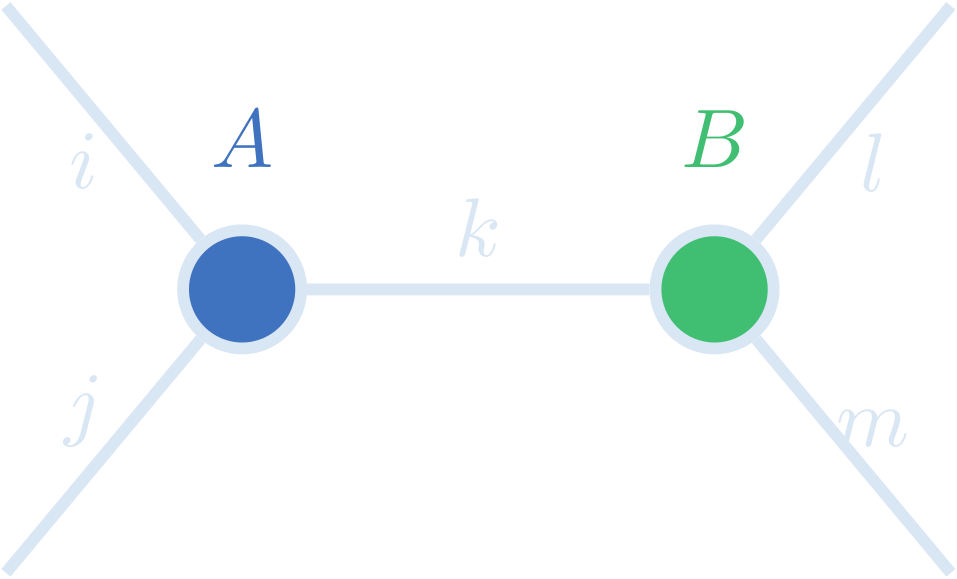
More generally, the tensor product of two matrices \(A, B\) is defined as a block matrix
\[\begin{equation*}
A \otimes B =
\begin{pmatrix}
A_{1,1} B & A_{1,2} B & \cdots & A_{1,n} B\\
A_{2,1} B & A_{2,2} B & \cdots & A_{2,n} B\\
\vdots & \vdots & \ddots & \vdots \\
A_{m,1} B & A_{m,2} B & \cdots & A_{m,n} B\\
\end{pmatrix}.
\end{equation*}
\]
Consider the CNOT matrix.
It creates a correlation between the two coins.
Quantum mechanics is similar, except that it uses
amplitudes.
Quantum (Pure) States
A quantum state is a unit vector of \(\complex^N\).
Finite dimensional spaces suffice for this course.
A qubit is a superposition of 0 and 1.
Quantum states are superposition of
possibilities.
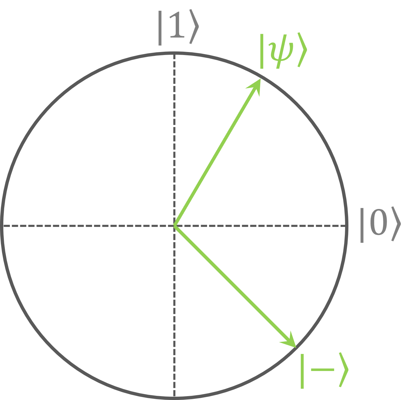
Dirac notation.
ket, bra (\(\ket{0}, \ket{1}, \ket{+},
\ket{-}, \ket{\psi}\)).
State Transformation
Unitary. \(U^\dagger U = I\).
Examples: \(I, X, Y, Z, H, S, T\),
CNOT, rotations.
\[\begin{equation*}
H = \frac{1}{\sqrt{2}}
\begin{bmatrix}
1 & 1\\
1 & -1
\end{bmatrix}.
\end{equation*}
\]\[\begin{equation*}
H \ket{0} = \ket{+}, H \ket{1} = \ket{-}.
\end{equation*}
\]
Why unitary? Unitary operators are the only operators that preserve
the length of vectors.
If \(\{ \ket{\lambda_i} \}\) form
an orthonormal basis, then we have
\[\begin{equation*}
\sum_j \ket{\lambda_j} \bra{\lambda_j} = I.
\end{equation*}
\]
Adjoints of operators
Let \(A\) be a linear operator on
a Hilbert space. There exists a unique operator \(A^\dagger\) such that for all \(\ket{v}, \ket{w}\),
\[\begin{equation*}
(\ket{v}, A \ket{w}) = (A^\dagger \ket{v}, \ket{w}).
\end{equation*}
\]
In the matrix form, \(A^\dagger\)
is the conjugate transpose of \(A\).
Eigenvalues and
Eigenvectors
\(A \ket{\lambda} = \lambda
\ket{\lambda}\).
Matrix \(A\) is
diagonalizable if \(A =
\sum_j \lambda_j \ket{\lambda_j}
\bra{\lambda_j}\) where \(\ket{\lambda_j}\) form an orthonormal set
of eigenvectors of \(A\).
Example: What is the eigenvalues and eigenvectors of \(X\)?
Spectral decomposition theorem
Theorem. Any normal operator \(A\) on space \(V\) is diagonalizable with respect to
some orthonormal basis of \(V\), and
vice versa.
Families of diagonalizable matrices
Matrix
Condition
Eigenvalues
Normal
\(A\) and \(A^\dagger\) commute
Complex
Hermitian
\(H = H^\dagger\)
Real
Unitary
\(U^\dagger U = I\)
Phase
Projection
\(P^2 = P, P = P^\dagger\)
\(\{0,1\}\)
Reflection
\(R^2 = I, R = R^\dagger\)
\(\{\pm 1\}\)
Tensor Products
\(A \otimes B\) is a block
matrix whose \(i,j\)-th block is
\(a_{i,j} B\).
\[\begin{equation*}
X \otimes Y =
\begin{bmatrix}
0 & 0 & 0 & -i\\
0 & 0 & i & 0\\
0 & -i & 0 & 0\\
i & 0 & 0 & 0
\end{bmatrix}
\end{equation*}
\]
Matrix Functions
For \(A = \sum_a a
\ket{a}\bra{a}\), define \(f(A) =
\sum_a f(a) \ket{a}\bra{a}\).
Example: \(\exp(A)\).
Four Postulates
State
The state of a closed quantum system can be
described by a unit vector in a Hilbert space (called the state
space).
Closed: no observer, no leak of information to the environment!
If a "particle" can be in one of the \(d\) possibilities from a finite set \(\Gamma\), the state space is \(\mathcal{H} = \complex^\Gamma\). That is,
to each possibility in \(\Gamma\), a
complex number (the amplitude) is assigned.
such that \(\norm{\ket{\psi}} =
\abs{\psi_1}^2 + \cdots + \abs{\psi_d}^2 = 1\).
Evolution
The discrete time evolution of the closed system can be described
by a unitary operator. If the state at time \(t_0\) is \(\ket{\psi_0}\), the state at time \(t_1\) can be obtained as
\[\begin{equation*}
\ket{\psi_1} = U \ket{\psi_0}.
\end{equation*}
\]
It also follows from the Schrödinger equation
\[\begin{equation*}
i \hbar \frac{\partial}{\partial t} \ket{\psi(t)} = H \ket{\psi(t)}.
\end{equation*}
\]
Take \(\hbar = 1\), the evolution
from \(t_0\) to \(t_1\) is
\[\begin{equation*}
U = \exp \bigl(-i H (t_1 - t_0) \bigr).
\end{equation*}
\]
Measurement
Composite system
The state of a composite system whose components have states \(\ket{\psi_1},
\ket{\psi_2}, \ldots, \ket{\psi_m}\) is the tensor product
state
Quantum measurements are described by a collection \(\{M_m\}\) of measurement operators. These
are operators acting on the system being measured and must satisfy
\[\begin{equation*}
\sum_m M_m^\dagger M_m = I.
\end{equation*}
\]
The index \(m\) refers to the
measurement outcomes that may occur.
(Compare the \(U^\dagger U = I\)
condition)
If the state of the system is \(\ket{\psi}\) immediately before the
measurement then the probability that result \(m\) occurs is given by
Quantum measurements are described by measurement operators \(\{M_m\}\) satisfying
\[\begin{equation*}
\sum_m M_m^\dagger M_m = I.
\end{equation*}
\]
The probability that \(m\)
occurs is \(\bra{\psi} M_m^\dagger M_m
\ket{\psi}\).
The post-measurement state given outcome \(m\) is proportional to \(M_m
\ket{\psi}\).
An observable is a Hermitian operator whose
eigenprojectors form a set of measurement operators indexed by the
eigenvalues.
\(Z\) is an observable, which
corresponds to the computational measurement \(\{\ket{a}\bra{a}\}\) with outcomes \((-1)^a\).
Global and Relative Phase
The global phase is not observable in quantum mechanics.
Quantum Circuits
How do we process information using the four postulates?
Classical Information
Review
Boolean functions, Boolean circuits, and Boolean formulas
A Boolean function is function \(f :
\{0,1\}^n \to \{0,1\}\).
There are \(2^{2^n}\) of them!
Simple Boolean functions: AND (\(\land\)), OR (\(\lor\)), NOT (\(\neg\)), NAND (\(\uparrow\)).
\(n = 1\) and \(n = 2\).
A Boolean circuit is a model of computation using gates and
wires.
Each gate has at most two inputs and one output;
The fan-out of a gate is unrestricted;
Fan-in 0 nodes correspond to input variables;
Fan-out 0 node(s) correspond to output(s).
A Boolean formula is a Boolean circuit where all gates have
fan-out at most \(1\).
Functional completeness
A set of Boolean functions \(f_i :
\{0,1\}^{n_i} \to \{0,1\}\) is functionally complete if the
functions "generate" every \(f : \{0, 1\}^n
\to \{0, 1\}\) for all \(n \ge
1\).
\(\{\text{AND}, \text{OR},
\text{NOT}\}\) is functionally complete.
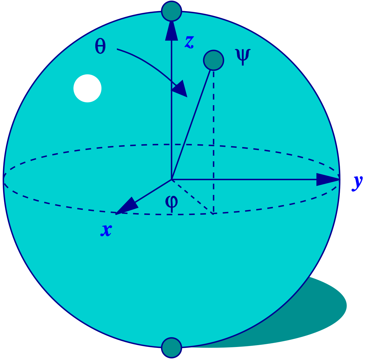
It would be more natural first to define the \(\vec{n} \cdot \vec{\sigma}\) operator for
any coordinate and define the pure state as its eigenvalue-\(1\) eigenstate.
It explains the \(\frac{\theta}{2}\) used to define the
state \(\ket{\psi}\).
Rotate!
Pauli Actions on the Bloch
Sphere
Pauli \(X\), \(Y\), \(Z\) rotate the Bloch sphere by angle
\(\pi\) along the \(x\), \(y\), \(z\) axis, respectively.
\[\begin{equation*}
\begin{split}
& H = \frac{1}{\sqrt{2}}
\begin{pmatrix}
1 & 1 \\
1 & -1
\end{pmatrix},\quad
S = \begin{pmatrix}
1 & 0\\
0 & i
\end{pmatrix},\\
& T = \begin{pmatrix}
1 & 0 \\
0 & e^{\pi i / 4}
\end{pmatrix}.
\end{split}
\end{equation*}
\]
Rotations through \(a = x, y,
z\) axis
\[\begin{equation*}
R_a(\phi) = \exp\Bigl( - \frac{\phi}{2} i \sigma_a \Bigr) =
\cos\frac{\phi}{2} I - i\sin\frac{\phi}{2} \sigma_a.
\end{equation*}
\]
In particular, \(R_z(\phi) =
\begin{pmatrix} e^{-\frac{\phi}{2} i} & 0 \\ 0 &
e^{\frac{\phi}{2} i} \end{pmatrix}\), and \(T\) is \(R_z(\pi / 4)\) up to a global
phase.
A projective measurement in the direction of \(\vec{n}\)
Note that \(\vec{n} \cdot
\vec{\sigma}\) is an observable.
Measurement operators
\[\begin{equation*}
M_b = \frac{I + (-1)^b\, \vec{n} \cdot \vec{\sigma}}{2},
\text{ for } b = 0, 1.
\end{equation*}
\]
Check that \(M_b\) is indeed
projective and \(M_0 + M_1 =
I\).
Detect Elitzur-Vaidman Bomb
Someone sends you a box, which is either a dud (empty box) or a
bomb attached to a quantum device that will trigger the explosion if
it measures a \(\ket{1}\) on the
photon sent in. Your task is to detect if there is a bomb inside.
Classical Method
Not very interesting
Send in \(\ket{+}\), Measure Output in \(\ket{\pm}\)
CNOT and single-qubit gates are all you need for universal
quantum computing.
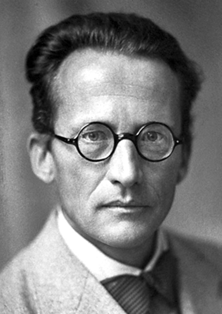
The Characteristic Trait
…, then they can no longer be described in the same way as before,
viz. by endowing each of them with a representative of its own. I
would not call that one but rather the characteristic trait
of quantum mechanics, the one that enforces its entire departure from
classical lines of thought. By the interaction the two representatives
[the quantum states] have become entangled.
The first index determines the sign; the second determines the
parity.
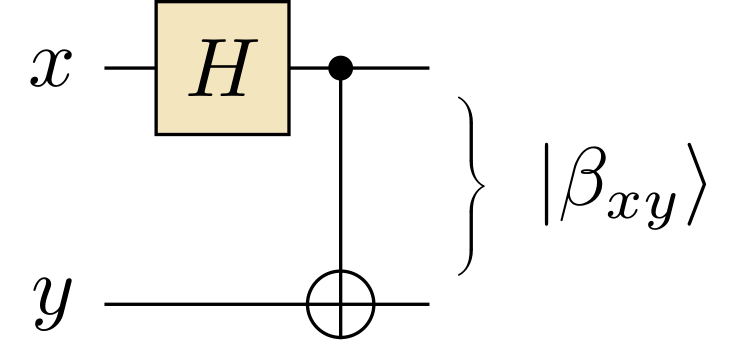
Prepare the Bell states
The Bell states are also known as the EPR states, and we often
use \(\ket{\text{EPR}}\) to denote
\(\ket{\beta_{00}}\).
Singlet state \(\ket{\beta_{11}}\) is an anti-symmetric
state.
The other three states are all symmetric and span the symmetric
subspace of the two-qubit state space.
Entanglement
It is easy to verify that this state is not a
product of single-qubit states!
A picture of entanglement.
Basic rules of quantum mechanics imply the
existence of EPR, arguably what troubled Einstein the most in quantum
mechanics! It is what he called the 'spooky action at a
distance'.
EPR Paradox
Consider two players Alice and Bob sharing an EPR state. Alice
brings her particle to the moon while Bob stays on earth.
Fact: If Alice measures her particle, she instantaneously
knows whether Bob's state is \(\ket{0}\) or \(\ket{1}\) (which Bob can confirm if he
performs the standard basis measurement).
Is it a big deal?
It is not very different from a pair of two perfectly correlated
classical bits.
A pair of gloves in two boxes.
EPR considers other possibilities: Alice can measure in a
different basis.
There is another way to open the box.
We have measured \(Z\) basis, what
about \(X\) measurement? That is,
what happens if Alice measures \(\ket{\pm}\)?
Method I. \(M_0 = \ket{+}\bra{+}
\otimes I\) and \(M_1 =
\ket{-}\bra{-}
\otimes I\).
The conclusion is that Alice will instantaneously know
whether Bob's post-measurement state is \(\ket{+}\) or \(\ket{-}\).
Superluminal Communication?
No!
Consider two situations. In the first, Alice measures in the
standard basis, she will obtain \(a=0,1\) with equal probability and Bob's
qubit collapses to \(\ket{a}\). In
the second, she measures in the Hadamard basis, she will obtain \(a={+},{-}\), with equal probability and
Bob's qubit collapses to \(\ket{a}\).
It looks as if Alice's measurement choice affects Bob's final
state! Would it allow Alice to send information
instantaneously to Bob?
What are the states of Bob in the two situations?
Bob's view and Alice's view.
The mixed state framework will help us to answer the question and
see why this won't allow superluminal communication.
Mixed States
Ensembles
In the first situation, Bob's state is in an equal distribution
over \(\ket{0},
\ket{1}\). In the second, it is an equal distribution over
\(\ket{+}\) and \(\ket{-}\). Can we
distinguish these two cases in quantum mechanics?
Let's generalize a little bit and consider a distribution of pure
states described by an ensemble\(\{(p_i, \ket{\psi_i})\}\). It means that
our knowledge of the quantum system says that it is in state \(\ket{\psi_i}\) with probability \(p_i\).
Consider a quantum measurement \(\{M_0,
M_1\}\) measuring the state ensemble. The probability that
\(a\) occurs is
the density matrix of the ensemble. The
probability is determined by the density matrix, so it makes sense to
use the density matrix to describe the state of the system.
Bob's Mixed State
We now go back to the EPR paradox. When Alice measures \(\ket{0}, \ket{1}\), Bob's state is also
\(\ket{0}\) or \(\ket{1}\), which Alice knows for sure as
it will be the same as her measurement outcome. But Bob does
not know the measurement outcome, so before Alice send the
outcome to him, his knowledge of the system is that it is \(\ket{0}\) or \(\ket{1}\) with equal probability. The
density matrix is
So even though the two ensembles look very different, the density
matrices in the two situations are the same. It means
that no measurement on Bob's system can tell the two cases apart. This
makes perfect sense as the state of Bob should not change when Bob has
done nothing to his system.
It explains why density matrix is more fundamental
then ensemble of quantum states.
No superluminal communication is possible using the strategy
above!
Density Matrix
Mathematically, a density matrix is positive
semidefinite and of trace \(1\) (iff
there is a corresponding ensemble). It is a description of the state
of a quantum system that is more general than state vectors for pure
states.
Any pure state \(\ket{\psi}\) has
a density matrix representation \(\rho =
\ket{\psi}\bra{\psi}\).
Conversely, given the density matrix \(\rho\), the expansion in the Pauli
operators basis gives a vector \(\vec{n} =
(n_x, n_y, n_z)\)
\[\begin{equation*}
n_a = \tr(\rho \sigma_a), \text{ for } a = x, y, z.
\end{equation*}
\]
Classical probability over a bit can be represented as diagonal
density matrices corresponding to the line segment between the north
and south poles.
Summarize: Things that can be identified with point \(\vec{n}\) on the sphere.
Measurement of Mixed Qubit
State
When we measure \(\rho = (I + \vec{n}
\cdot \vec{\sigma})/2\):
With probability \(\tr(\rho\,
\ket{0}\bra{0}) = (1 + n_z) / 2\), the measurement outcome is
\(0\) and the state collapse to \(\ket{0}\bra{0}\);
With probability \(\tr(\rho\,
\ket{1}\bra{1}) = (1 - n_z) / 2\), the measurement outcome is
\(1\) and the state collapse to \(\ket{1}\bra{1}\).
Partial Trace
Partial Trace and
Purification
What is the state of \(A\) given
the state of \(AB\)? We cannot answer
the question in the pure state framework, and we can now with density
matrices.
Partial Trace
Let \(\rho_{AB}\) the joint state
of \(A\) and \(B\) systems. What is the state of \(B\) only? Is there a density matrix
associated with system \(B\) given
that we know the state of both \(A\)
and \(B\)?
We need an effective representation of the state on \(B\) so that measurement only depends on
this reduced state (not the joint state).
Let \(M\) be a measurement
operator; the probability its outcome occurs is
Consider subspace \(K\) spanned by
all vectors orthogonal to \(\ket{e_1}\).
We prove that \(K\) is an
invariant subspace of \(A\). Suppose \(\ket{\psi} \in K\), we have \(\bra{e_1} A \ket{\psi} = \lambda_1 \langle e_1 |
\psi \rangle = 0\). Use induction to complete the proof.
In standard textbooks, it says that \(A =
UDU^\dagger\). Using Dirac notation, we write it as
\[\begin{equation*}
A = U \bigl( \sum_j \lambda_j \ket{j}\bra{j} \bigr) U^\dagger.
\end{equation*}
\]
In this form, \(\ket{e_j} =
U\ket{j}\) will be the eigenvectors of \(A\), and we write
\[\begin{equation*}
A = \sum_j \lambda_j \ket{e_j}\bra{e_j},
\end{equation*}
\]
and \(\ket{e_j}\)'s are
orthonormal.
Measurement
Projective measurements
Measurement operators are projectors such as \(\ket{0}\bra{0}\) and \(\ket{1}\bra{1}\).
Note that \(\ket{\psi}\bra{\psi}\)
is the projector to the span of \(\ket{\psi}\).
A set of projectors \(\{P_j\}\)
form a projective measurement if \(\sum_j
P_j = I\).
General measurement satisfies \(\sum_j M_j^\dagger M_j = I\)
When we don't care about the post-measurement state, we
consider measurement operators \(N_j =
M_j^\dagger M_j \ge 0\).
The completeness condition is \(\sum_j
N_j = I\).
The probability that \(j\) occurs
is \(\tr(N_j \rho)\).
They are called positive-operator valued measure (POVM).
Entanglement Revisit
Schmidt Decomposition
(Schmidt Decomposition). For a bipartite pure
quantum state \(\ket{\psi_{AB}}\), we
can write
Hint: Consider the singular value decomposition of matrix \((\psi_{j,k})\).
EPR as a mirror!
For any matrix \(U\):
\[\begin{equation*}
(U \otimes I ) \sum_j \ket{j,j} = (I \otimes U^T) \sum_j \ket{j,j}
= \sum_{i,j} U_{i,j} \ket{i,j}
\end{equation*}
\]
\(\lambda_j\)'s are called the
Schmidt coefficients
What are the Schmidt coefficients of the Bell
states?
How about product states?
Thanks to this theorem, the theory of pure bipartite
entanglement is well established.
Nielsen's Theorem
Local operation and classical communication (LOCC)
Nielsen's Theorem
Let \(\ket{\psi}\) and \(\ket{\phi}\) be two entangled states on
systems \(A,B\). Their Schmidt
coefficients are \(\lambda =
(\lambda_j)\) and \(\gamma =
(\gamma_j)\) respectively.
Theorem (Nielsen). There is an LOCC transforming
\(\ket{\psi}\) to \(\ket{\phi}\) if and only if the
majorization condition \(\lambda \prec
\gamma\) holds.
The condition \(\lambda \prec
\gamma\) is that for all \(k\)
Entanglement is a resource for many quantum information processing
tasks
Now utilized for good at a distance of at least 1200km (Mozi
satellite).
Quantum entanglement—physics at its strangest—has moved out of this
world and into space. In a study that shows China's growing mastery of
both the quantum world and space science, a team of physicists reports
that it sent eerily intertwined quantum particles from a satellite to
ground stations separated by 1200 kilometers, smashing the previous
world record. (Science,
15 JUN 2017)
What is Information?
A qubit is a unit of quantum information storing the quantum state
of a two-level physical system.
Quantum information is more general than classical information. We
can store a bit in a qubit. But to store a qubit, it may require an
infinite number of bits.
Distingish (Mixed) Quantum
States
Consider an encoding \(a \mapsto
\rho_a\) for \(a=0, 1\).
Promise: The system is in one of the two states \(\rho_0\) and \(\rho_1\),
Problem: Decide which is the case.
Measurement is the only bridge between the quantum and
classical worlds. So we use a measurement with measurement operators
\(M_0\) and \(M_1\)
The optimal \(M_0\) minimizes
\(\Tr(M_0 (\rho_1 -
\rho_0))\)
In the qubit case, we write \(\rho_b
= (I + \vec{v}_b \cdot \vec{\sigma}) / 2\), and \(\rho_0 - \rho_1 = \vec{v} \cdot
\vec{\sigma}\) for \(\vec{v} =
(\vec{v}_0 -
\vec{v}_1)/2\). The optimal \(M_0\) should be
The minimal error probability is therefore \((2 - \lVert \vec{v}_0 - \vec{v}_1
\rVert )/ 4\).
If two states \(\ket{u}\) and
\(\ket{v}\) of a qubit are
orthogonal, there is a projective measurement to tell them apart.
If two states are co-linear, they are indistinguishable.
The amount of information one can store and reliably read from a
qubit is only a single bit.
The states \(\ket{0}\) and \(\ket{+}\) are different but not perfectly
distinguishable.
Non-orthogonality is the key issue.
What is information? What is quantum information?
We can store the whole Internet in a single qubit, but we cannot
reliably read information out.
Holevo Bound
A. Holevo
For a quantum state \(\rho\),
its von Neumann entropy is \(S(\rho) = -\tr (\rho
\log(\rho))\).
The eigenvalues of \(\rho\) form a
probability distribution whose Shannon entropy equals
the von Neumann entropy \(S(\rho)\).
Mutual information \(H(X{\,:\,}Y) = H(X)
+ H(Y) - H(XY)\).
Theorem. Let \(\{(p_x,
\rho_x)\}\) be an ensemble of states. Alice prepares \(\rho_x\) with probability \(p_x\) and sends it to Bob. Bob measures
the state and gets outcome \(y\).
Then the mutual information (accessible information)
between \(X\) and \(Y\) satisfies
We will prove a poor man's version of Holevo's
theorem.
Let \(X\) be a uniformly
distributed random variable taking values in \([N]\). Consider an encoding of classical
information \(x \mapsto \rho_x\) into
quantum systems of \(n\) levels. For
all measurement (POVM) \(\{M_m\}\),
the probability that the measurement correctly guesses \(x\) is
There is no unitary transformation \(U\) that can map any \(\ket{\psi} \ket{0}\) to \(\ket{\psi} \ket{\psi}\).
Compute the inner product.
Note: \(\ket{0}\) and \(\ket{1}\) can be cloned using the CNOT
gate.
Tomography
State Tomography
Given a large number of i.i.d samples of quantum state \(\rho\), find the density matrix for \(\rho\).
In the single-qubit case, \(I\), Pauli \(X\), \(Y\), \(Z\) form an orthonormal basis, so
\[\begin{equation*}
\rho = \frac{\tr(\rho)I + \tr(X \rho) X + \tr(Y \rho) Y + \tr(Z
\rho) Z}{2}.
\end{equation*}
\]
For example, to estimate \(\tr(Z
\rho)\), we need to measure \(\rho\) in the \(Z\) basis multiple times, obtaining \(z_1, z_2, \ldots, z_m \in \{\pm 1\}\).
Then \((\sum_i z_i) / m\) is an
empirical estimate of \(\tr(Z
\rho)\).
Note that the standard deviation is \(1/\sqrt{m}\) and so we need to repeat
about \(O(1/\eps^2)\) times to have
\(\eps\) precision.
where the summation goes over \(n\)-qubit Pauli operators.
Check that \(I\) and Pauli
operators form a basis also in the multiple qubit case.
But it's a summation of \(4^n\) terms!
In the lab, it would take days to tomography a system of more than
10 qubits.
Theorem. The sample complexity for tomography is
\(\tilde{\Omega}(d^2/\eps^2)\), where
\(d\) is the dimension and \(\eps\) is the precision in the so called
trace distance.
To make things worse, each term needs high precision for the
triangle inequality to give meaningful bounds.
There are \(4^n\) small real
numbers \(\tr(\rho P)\), and we have
to ensure that their error sum is still controlled.
How do we even know the quantum device works as expected when
tomography of its state is impractical?
Example: Tomography
of the Singlet State
We need to estimate 15 real numbers \(\mu_P =
\tr(\ket{\beta_{11}}\bra{\beta_{11}} P)\) for non-identity
two-qubit Pauli operators \(P\).
I
X
Y
Z
I
0
0
0
X
0
-1
0
0
Y
0
0
-1
0
Z
0
0
0
-1
For \(P = XX, YY, ZZ\), \(\mu_P = -1\),
For all other \(P\), \(\mu_P = 0\).
Note that in this simple case, it suffices to check the \(XX, YY, ZZ\) average values in the first
case to certify that the state is the singlet state.
The singlet state is the unique state stabilized by \(-XX\) and \(-ZZ\).
Lecture 6: Teleportation
Teleport!
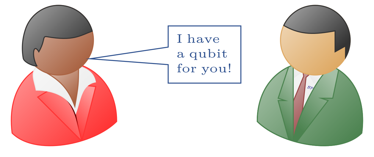
The Setup
We have two players, Alice and Bob.
Alice and Bob share an EPR state.
Alice also has an input qubit given in some unknown state \(\ket{\psi}\).
Classically, there are two methods.
Physically transfer
Copy and send
She wants to transfer this qubit to Bob using classical
communication only.
Even if Alice knows the description of the state \(\ket{\psi}\), for example, maybe she
prepared the state using a circuit on her own, the task is still
really challenging.
To describe the state, we need to specify two real
numbers!
The teleportation protocol needs to transfer
two bits from Alice to Bob by consuming the shared EPR state.
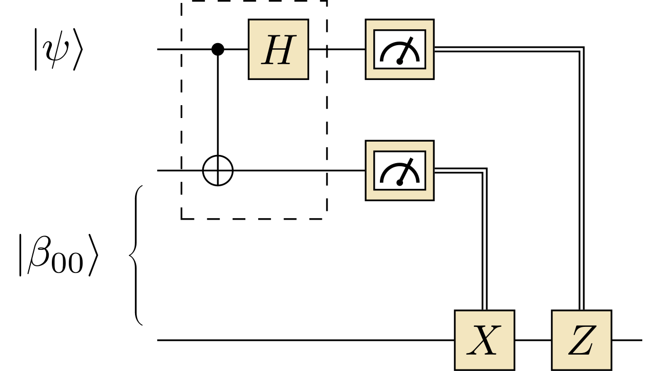
The Protocol
We name the qubit in the shared EPR state between Alice and Bob
and the input qubit as A, B, and C, respectively.
Alice measures the projective measurement defined by the four Bell
states on A and C, let \(a, b\) be
the outcome bits;
Alice sends the classical outcome \(a,
b\) to Bob;
Bob applies \(Z^a X^b\) to
B.
The Bell states form an orthonormal basis for the two-qubit
system \(AC\).
How Did the Authors
Come Up With This?
The protocol is simple but very hard to find and only
discovered in 90's (quantum mechanics was completely established in
the 30's).
Teleporting an unknown quantum state via dual classical and
Einstein-Podolsky-Rosen channels
[C. Bennett, G. Brassard, C. Crépeau, R. Jozsa, A. Peres and W.
Wootters, '93]
The Origins of Quantum Teleportation - Charles Bennett
What is it that they don't have that they need that would enable
them to do as well if they were in separate locations than if they
were in the same location.
… So then we realized that by sharing entanglement between the two
observers and by permitting them to communicate, you could simulate
being in the same place.
If it is the first you see this, you may feel a bit confused about
how we get the above expansion. The key is to use linearity to do this
on product state terms and take the sum. Alternatively, you may
consider multiplying
\[\begin{equation*}
I = \sum_{i,j} \ket{\beta_{ij}}\bra{\beta_{ij}}_{AC} \otimes I_B
\end{equation*}
\]
If the measurement has outcome \(a,
b\), the state on \(B\) after
correction is
The Bell measurement is the same as measuring the \(XX\) and \(ZZ\) observables.
We can measure both as they are
compatible.
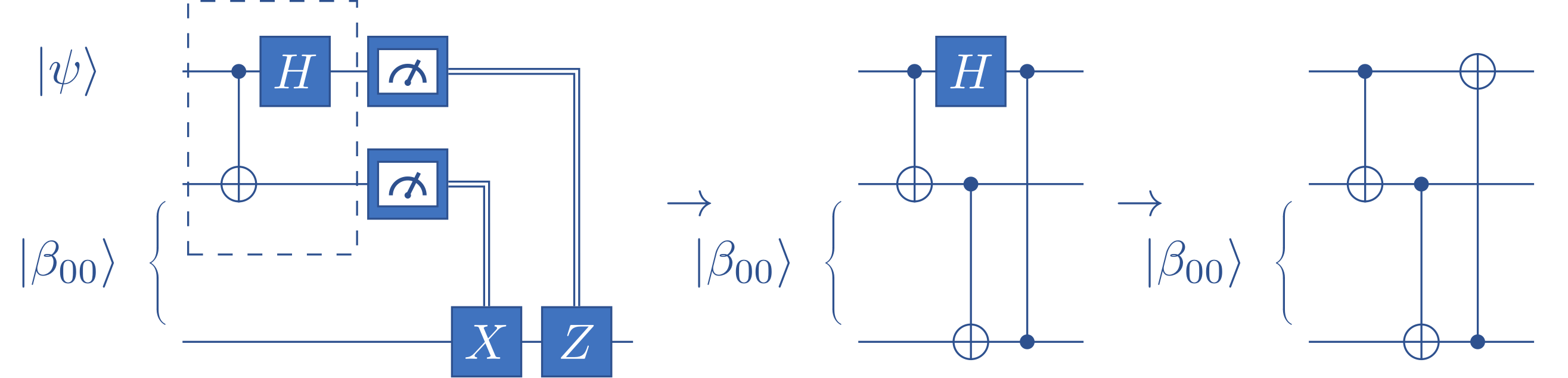
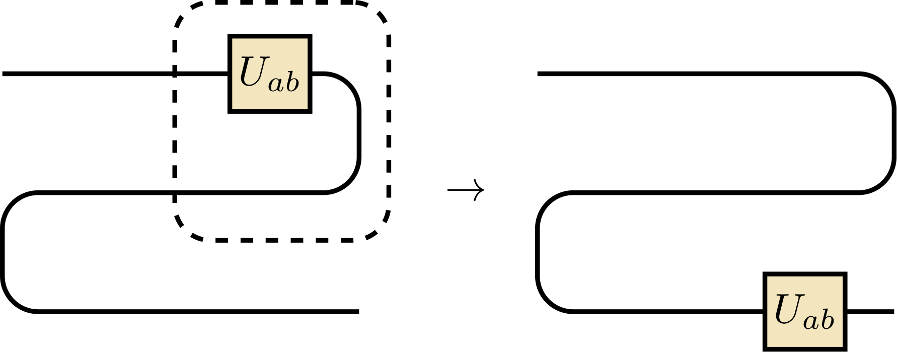
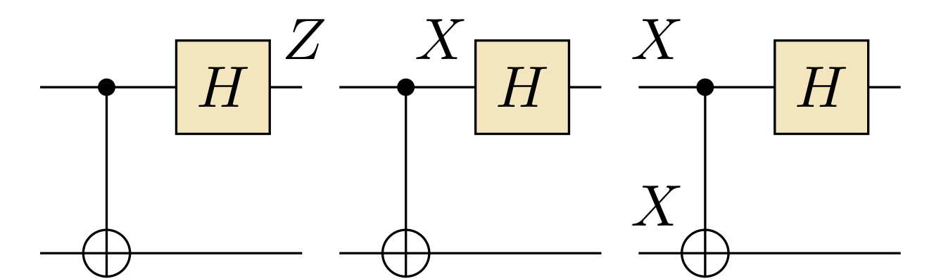
Back propagation of operators
Teleportation is explained in the stabilizer framework.
It is enough to make sure \(X\)
and \(Z\) measurements are
recovered.
Discussions
Understanding Teleportation
What if the input state on C is part of a larger system \(CD\) and the state on \(CD\) is \(\ket{\psi}_{CD}\)?
After the teleportation, the state on \(BD\) is \(\ket{\psi}\). That is, the correlation
(entanglement) between \(CD\) is
preserved and teleported to \(BD\)!
A special case is when \(\ket{\psi} =
\ket{\text{EPR}}\), another EPR pair.
It is known as the Entanglement Swapping
protocol.
Would teleportation allow faster-than-light quantum
transmission?
Bob has one-time padded quantum information without the two
bits.
Would teleportation allow the cloning of quantum
information?
Did the Bell measurement learn anything about
the input state?
Superdense Coding
A dual problem of teleportation
Alice and Bob share an EPR state;
Alice gets two bits \(a, b\) as
input;
Alice applies \(X^a Z^b\) on her
half of the EPR state and sends her qubit to Bob;
Bob performs Bell measurement to get \(a, b\).
The four Bell states can be transformed to each other
locally.
The four Bell states are orthogonal to each other and are
therefore perfectly distinguishable.
A scheme for sharing classical secrets (2 bits) among two
players (each holding one qubit).
Question: is it possible to share quantum secrets?
Entanglement as a Resource
Teleportation, superdense coding, and many other protocols use
EPR and entanglement as resource, without which the protocols cannot
be carried out.
They motivated the study of entanglement as a new type of
resource.
How do we quantify the amount of entanglement needed for a certain
task?
Mixed State Entanglement
(Skip)
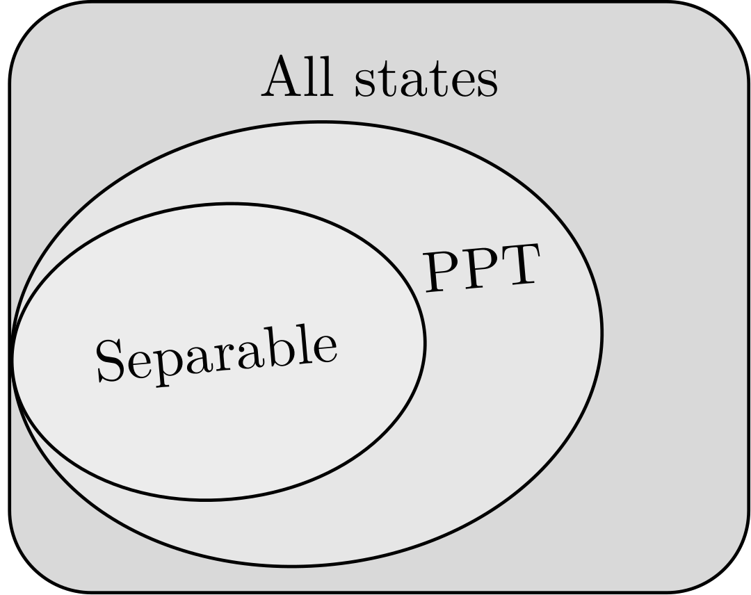
A mixed state \(\rho_{AB}\) is
said to be separable if there is an ensemble of the form
\(\bigl\{ \bigl( p_i, \rho_{A}^{(i)} \otimes
\rho_{B}^{(i)} \bigr)
\bigr\}_{i=1}^k\) such that
[M. Ying, L. Zhou, and Y. Li, Reasoning about Parallel Quantum
Programs, '18], [C. Piveteau and D. Sutter, Circuit Knitting with
classical communication, '22]
Peres PPT Condition (Skip)
How to check if a mixed state is separable or not?
Bound entanglement: entangled states which cannot be distilled
exist!
[Horodecki\(^3\), Mixed-state
entanglement and distillation, 1998]
Applications and Extensions
Quantum networks
Teleportation empowers entanglement swapping and quantum
repeaters.
Gate teleportation
[Aliferis and Leung, Computation by measurements: a unifying
picture, 2014]
Port-based teleportation
Lecture
7: Quantum Circuits and Early Quantum Algorithms
Quantum Circuits and
Universality
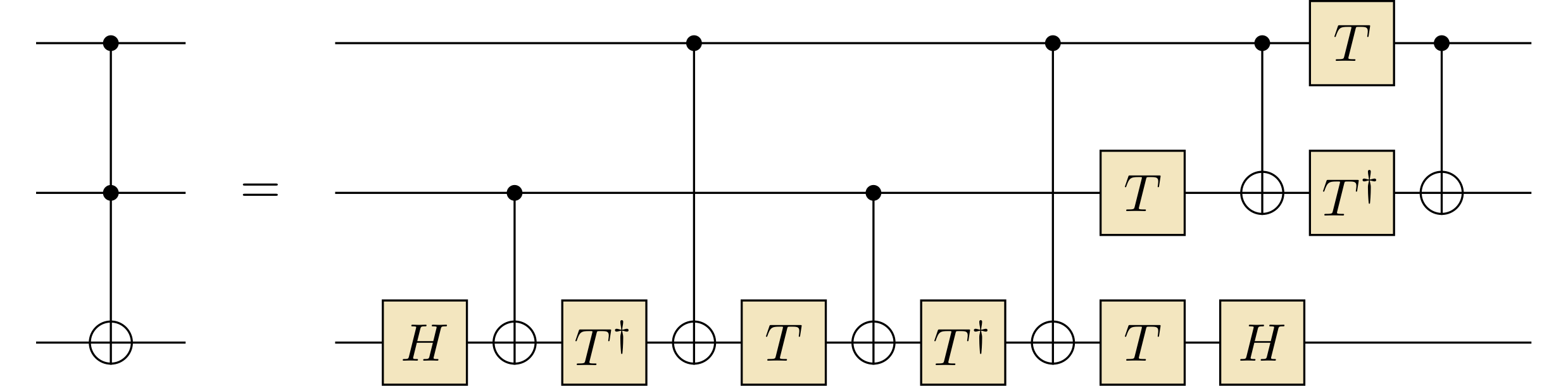
Toffoli and Fredkin
We have seen many quantum gates such as \(H\) and CNOT. We now introduce two
three-qubit gates called Toffoli and Fredkin.
Toffoli
\[\begin{equation*}
\mathrm{Toffoli}: \ket{a, b, c} \mapsto \ket{a, b, c \oplus a b}.
\end{equation*}
\]
Fredkin
\[\begin{equation*}
\mathrm{Fredkin}: \ket{a, b, c} \mapsto
\begin{cases}
\ket{a, b, c} & \text{ if } a = 0,\\
\ket{a, c, b} & \text{ if } a = 1.
\end{cases}
\end{equation*}
\]
Both Toffoli and Fredkin are classically
universal.
Simulate \(\mathrm{NAND}\) using
Toffoli.
Reversible Computation
Reversible classical computation and Landauer's principle
Energy consumption and irreversibility in computation
In the scenario where a computer erases bit of information, it
results in the dissipation of energy into its surrounding environment.
The minimum amount of energy that is released is proportional to \(k_B T \ln 2\), where \(k_B\) is Boltzmann's constant and \(T\) denotes the temperature of the
environment.
Does computation have to consume energy?!
It's possible to perform classical computation reversibly (using
Toffoli or Fredkin).
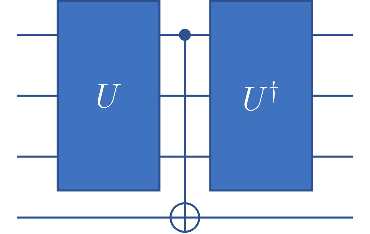
Uncompute technique
Clean the computational garbage!
Universal Gate Sets
A set of quantum gates is universal if all other unitary
operators can be generated exactly (or approximately) from that
set.
All gates are in \(\mathrm{SU}(d)\)
For any \(U \in \mathrm{SU}(d)\),
there is product of elements in the set that approximates \(U\).
Quantum computers are digital.
Approximation in the sense of the following distance
Complex numbers are essential for quantum mechanics but not for
quantum computing.
With an extra qubit, it is possible to map a circuit \(U\) with complex entries to a circuit
\(V\) with real entries.
Trick: \(a + bi \mapsto \begin{bmatrix}a
& b \\ -b & a\end{bmatrix}\).
Solovay-Kitaev Theorem
According to Wikipedia, it was first announced by Robert M. Solovay
in 1995 and independently proven by Alexei Kitaev in 1997.
Let \(G\) be a universal gate set
for \(\mathrm{SU}(d)\). Then there is
a constant \(c\) such that any
unitary in \(\mathrm{SU}(d)\) can be
approximated to error \(\eps\) using
a product of elements in \(G\) of
length \(\log^c(1/\eps)\).
Lemma. Let \([U,V] =
UVU^{-1}V^{-1}\) be the group commutator of \(U, V\) and let \(S_\eps\) be \(\{ U \in \mathrm{SU}(2) : \norm{I - U} \le \eps
\}\). If \(\Gamma\) is an
\(\eps^2\)-net for \(S_\eps\), then \([\Gamma, \Gamma] = \{ [U, V] \mid U, V \in
\Gamma \}\) is an \(\eps^3\)-net for \(S_{\eps^2}\).
Note that the lemma is not easy to use iteratively as the
scaling of \(\eps\)-net and the size
of the neighborhood of the identity do not match the initial
condition.
The closedness condition under inverse is not needed
anymore.
Subadditivity of Errors
Suppose \(U_i, V_i\) are unitary
operators satisfying \(\norm{U_i - V_i} \le
\eps\) for all \(i = 1, 2, \ldots,
t\). Then
This means that for a circuit of \(m\) gates using one gate set can be
transformed to a circuit of size \(m
\polylog(m/\eps)\) using one other gate where the total
approximation error is \(\eps\).
Early Quantum Algorithms
Superposition of Function
Calls
Let \(f : \X \rightarrow \Y\)
be a function that we know how to efficiently implement
classically.
This implies that we can efficiently perform the following
transform
Any classical algorithm (deterministic or randomized) needs
\(n\) queries.
The final answer consists of \(n\)
bits, and one classical query learns at most \(1\) bit of information.
Simon's Algorithm: Problem
Statement
Simon's algorithm is the main inspiration for Shor's factoring
quantum algorithm.
It shows that quantum computers are provably exponentially more
efficient (in terms of the number of queries) than
bounded-error randomized algorithms.
Simon's problem setup:
Oracle \(f: \{0,1\}^n \rightarrow
\{0,1\}^n\) satisfies that \(f(x) =
f(x')\) if and only if \(x =
x'\) or \(s + x = x'\)
for some hidden secret \(s \ne
0\).
Problem: Find \(s\).
Note that the function \(f\)
outputs multiple bits now, and it is a \(2\)-to-\(1\) function.
Simon's Algorithm
For \(i=1, 2, \ldots, O(n)\) do:
Prepare state \(\sum_{x} \ket{x}_A
\ket{f(x)}_B\);
Measure register \(B\);
Apply \(H^{\otimes n}\) and
measure all qubits in \(A\) to get
\(y^{(i)}\);
The measurement will output a random \(y\) such that \(s \cdot y = 0\).
Step 1.2 is not necessary.
Simon's Algorithm: Analysis
Each \(y^{(i)}\) is sampled
independently among those satisfying \(s \cdot
y^{(i)} = 0\).
To determine \(s\), we need to
have \(n-1\) linearly independent
\(y^{(i)}\)'s.
If the dimension of \(\text{span}(y^{(1)}, y^{(2)}, \ldots,
y^{(i-1)})\) has rank \(k <
n-1\), then the probability that \(y^{(i)}\) is not in the span is \(1 -
\frac{2^{k}}{2^{n-1}} \ge \frac{1}{2}\). This implies that the
algorithm runs in \(O(n)\) iterations
with high probability.
Simon's algorithm queries the oracle \(O(n)\) times.
Yet any classical algorithm needs \(\Omega(\sqrt{2^n})\) queries!
Simon's Algorithm:
Classical Bounds
Upper bound: By the birthday paradox, we expect to find \(x, x'\) such that \(f(x) = f(x')\) after \(O(\sqrt{2^n})\) queries.
Lower bound: Any classical (randomized or deterministic)
algorithm needs \(\Omega(\sqrt{2^n})\) queries.
We say that a sequence \(x_1, x_2,
\ldots, x_k\) is bad if there is no collision.
This excludes at most \(k \choose
2\) possible \(s\)'s.
For all \(k \ll \sqrt{2^n}\),
the probability that \(x_1, x_2, \ldots,
x_k\) is bad can be bounded as
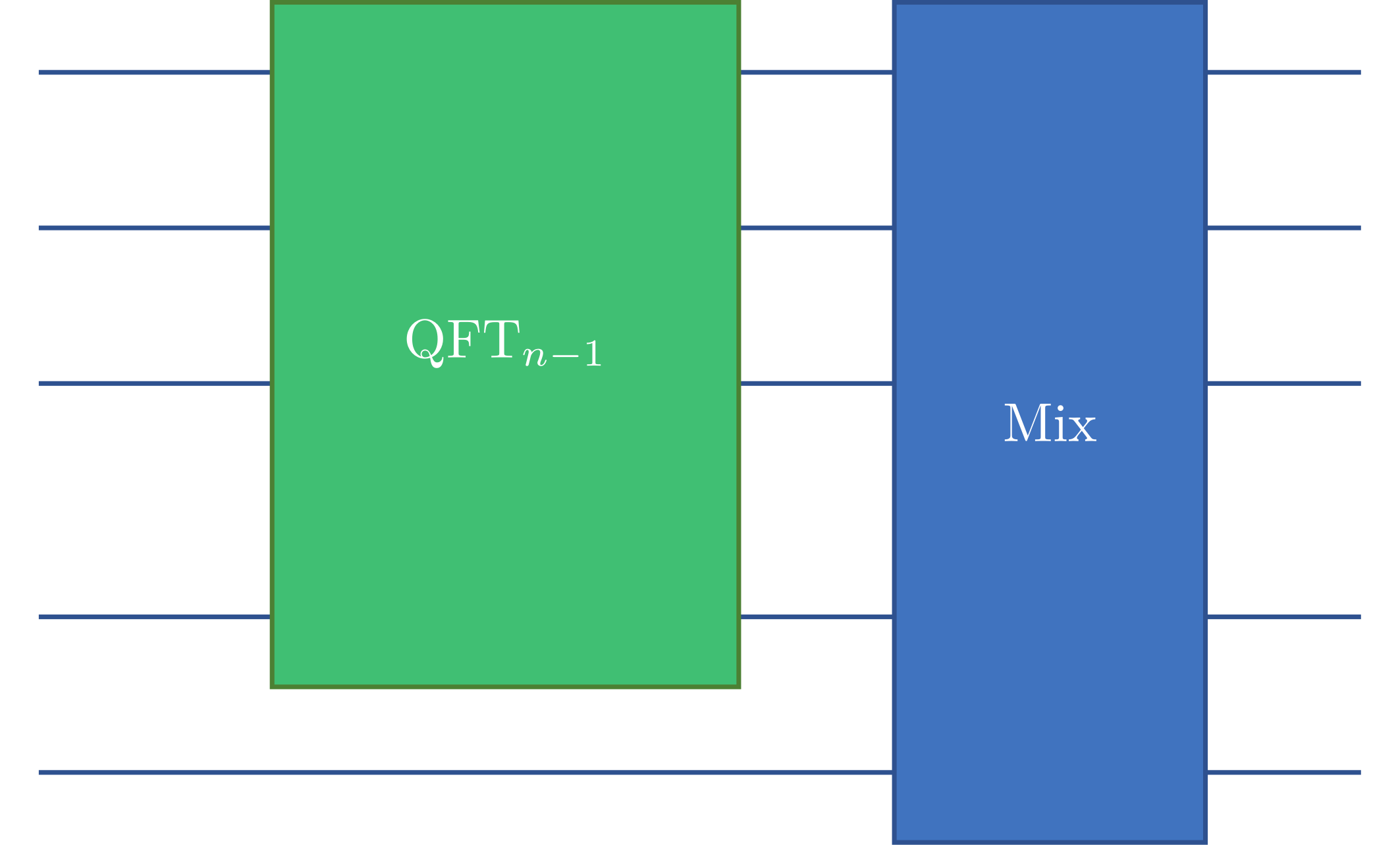
Move the last qubit to the first by SWAP gates, and we have
\(\ket{\hat{f}}\).
The last step is needed because we need \(\hat{f}(0y)\) and \(\hat{f}(1y)\).
Remarks on QFT
We have shown an efficient implementation of QFT.
Complexity is \(n^2\) or \(\log^2 N\).
A result shows that, if small rotations are omitted, QFT still
works approximately and has complexity \(n
\log n\).
Do not expect it to be useful in most problems
of signal processing!
You cannot read out the values of the amplitudes.
Lecture 8: Quantum Algorithms
II
Course Projects
Project Guidelines
You may select one of the provided topics and work in a group of up
to three students. While not mandatory, students are strongly
encouraged to pursue projects that contribute something novel, whether
through a new perspective, innovative methods, or original
algorithms.
Topic Selection Rules
Each topic can be chosen by at most two groups. Selection is on a
first-come, first-served basis (先到先得).
After making your choice, please contact the teaching assistant via
WeChat as soon as possible to secure your topic.
Contribution statement
The final submission must explicitly state each team member’s role,
responsibilities, and specific contributions (e.g., theoretical
analysis, implementation, experiments, writing, etc.).
Evaluation Criteria
Your project will be evaluated based on the following
components:
Understanding
Demonstrate a thorough comprehension of the topic, including its
background, key concepts, and relevant techniques.
(If applicable) Discuss recent advancements in the field, citing
relevant literature.
Writing (Research Paper Submission) Your written submission
should follow a structured research paper format, including:
Introduction – Provide context,
problem motivation, and a high-level summary of your
contributions.
Preliminaries – Define key
notations, assumptions, and foundational concepts.
Main Technical Content – Present
your core methodology, analysis, or findings with rigor.
Summary & Discussion –
Conclude with key takeaways, limitations, and directions for future
work.
Submission Timeline:
A draft must be submitted before
the presentation.
A final polished document is due
before Week 18.
In the final submission, please clearly state your individual
contributions to the project.
Presentation (Week 16)
Prepare clear, well-organized slides to effectively communicate
your work.
Emphasize key insights, methodology, and results.
Engage the audience with a logical flow and confident
delivery.
Originality
Submissions that introduce novel ideas, techniques, or
near-publishable results will be highly rewarded.
Creativity and innovation in problem-solving are strongly
encouraged.
Phase estimation is a powerful quantum algorithmic subroutine
used in many other quantum algorithms.
Phase Estimation
To get an \(m\)-bit estimate
of \(\phi\), the phase estimation
procedure performs the following with \(n =
m + O(\log(1/\eps))\),
Prepare state \(\displaystyle
\frac{1}{\sqrt{N}}
\sum_{x\in\X} \ket{x} \ket{\phi}\);
Apply unitary \(\displaystyle
\sum_{x\in\X} \ket{x}\bra{x} \otimes
U^x\), and the state becomes \(\displaystyle \frac{1}{\sqrt{N}} \sum_{x\in\X}
e^{i\phi x} \ket{x}\ket{\phi}\);
Apply an inverse quantum Fourier transform on the first
register.
If \(\phi = 2\pi y / 2^n\) for
some \(y\in \X\), the state in the
first register before the inverse Fourier transform is \(F \ket{y}\).
The first register is a good approximation of \(\phi/2\pi\).
The approximation will have \(m\) bits of precision with probability at
least \(1-\eps\).
If \(n = m\), the outcome is the
best \(n\)-bit approximation with
probability at least \(4/\pi^2\).
Discrete Logarithm and
Diffie-Hellman
2015 Turing Award
New directions in cryptography
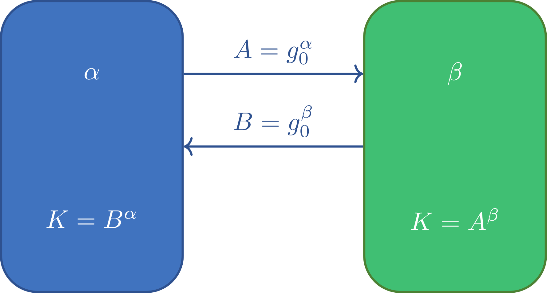
Given a cyclic group\(G =
\langle g_0 \rangle\) generated by \(g_0\) and an element \(h\in G\), the size \(N=\abs{G}\) is known.
The discrete logarithm \(\log_{g_0}
h\) of \(h\) in \(G\) with respect to \(g_0\) is the smallest non-negative
integer \(\alpha\) such that \(g_0^\alpha = h\).
Important for classical cryptography (Diffie-Hellman key
exchange)!
We can completely break the protocol, if we can solve the
discrete logarithm for \(A\) and
\(B\), the two messages exchanged by
the players,
Yet, no efficient classical algorithm is known.
Quantum Attack on
Diffie-Hellman
We attack the protocol by giving a quantum algorithm for
computing the discrete logarithm of a given \(h\).
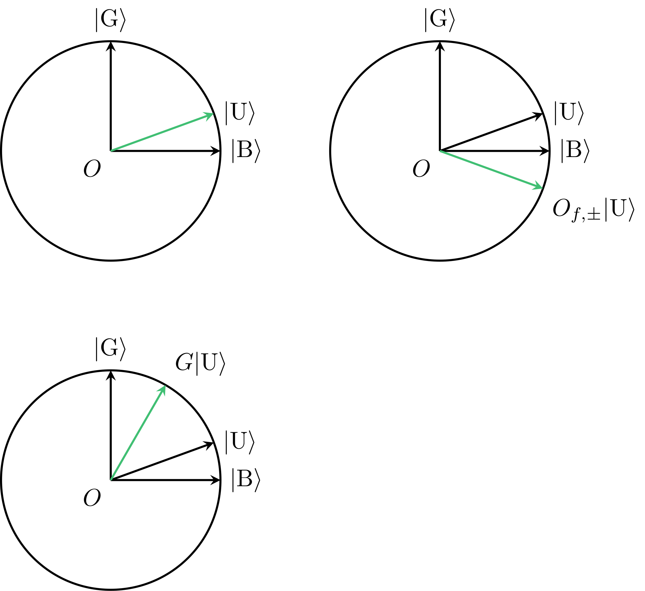
The Grover iterate consists of two reflections which generate a
rotation of \(2\theta\).
After \(k\) iterations, the
state is \(\sin\bigl((2k+1)\theta \bigr)\,
\ket{\mathrm{G}} + \cos\bigl((2k+1)\theta \bigr)\,
\ket{\mathrm{B}}\).
Choose \(k \approx
\frac{\pi}{4\theta} = O(\sqrt{N})\) as \(\sin\theta \le \theta\).
Amplitude Amplification
Setup the starting state \(\ket{\mathrm{U}} = \mathcal{A}
\ket{0}\);
Repeat the following for \(O(1/\sqrt{p})\) times:
Apply \(O_{f, \pm}\);
Apply \(\mathcal{A}R\mathcal{A}^{-1}\);
Measure.
A Boolean function \(f: X \to
\{0,1\}\) partitions \(X\)
into good and bad elements.
Suppose there is a quantum algorithm \(\mathcal{A}\) with no intermediate
measurements starting from \(\ket{0}\) finds a good element with
probability \(p\).
The amplitude amplification algorithm finds a good element with
\(O(1/\sqrt{p})\) calls to \(\mathcal{A}\) and \(\mathcal{A}^{-1}\).
Grover's algorithm is the special case where \(\mathcal{A} = H^{\otimes n}\).
Oblivious Amplitude
Amplification
Let \(U\) and \(V\) be unitary matrices and let \(\theta \in (0, \pi/2)\). Suppose that for
an \(n\)-qubit state \(\ket{\psi}\),
\[\begin{equation*}
U \ket{0^k}\ket{\psi} = \sin(\theta) \ket{0^k} V \ket{\psi} +
\cos(\theta) \ket{\Phi^\perp},
\end{equation*}
\]
where \(\ket{\Phi^\perp}\)
satisfies \((\bra{0^k} \otimes I)
\ket{\Phi^\perp} = 0\). Then there is a unitary \(W\) that uses \(U\), \(U^\dagger\)\(\ell\) times and a few simple gates,
\[\begin{equation*}
W \ket{0^k}\ket{\psi} = \sin((2\ell+1) \theta) \ket{0^k} V
\ket{\psi} +
\cos((2\ell+1) \theta) \ket{\Phi^\perp}.
\end{equation*}
\]
Oblivious: We don't need to reflect through \(\ket{\psi}\) which is required in
standard AA!
Quantum Hamiltonian
Simulation
Motivation
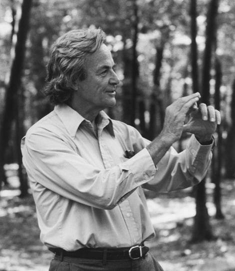
R. Feynman
… nature isn't classical, dammit, and if you want to make a
simulation of nature, you'd better make it quantum mechanical, and by
golly it's a wonderful problem, because it doesn't look so easy.
Simulating physics with computers (Feynman, 1981)
Analog simulation: Build a physical system whose Hamiltonian
effectively models the desired target system.
Digital simulation: Build a universal, fault-tolerant quantum
computer and run a quantum circuit/program to approximate the dynamics
of the target system
Hamiltonian Simulation
The Schrödinger equation is
\[\begin{equation*}
i\frac{\dif}{\dif t} \ket{\psi(t)} = H \ket{\psi(t)},
\end{equation*}
\]
where \(H\), mathematically a
Hermitian matrix of size \(2^n\) by
\(2^n\), is called the Hamiltonian of
the system and, as the equation says, it governs the dynamics of a
system.
It characterizes the energy of the system. If the state of the
system is \(\ket{\psi}\), the energy
is \(\bra{\psi} H
\ket{\psi}\).
We have \(\ket{\psi(t)} = U_t
\ket{\psi(0)}\) for unitary operator \(\displaystyle U_t = e^{-i H
t}\).
Give Hamiltonian \(H\) and
time \(t\), find a quantum
circuit\(U\) consisting of \(\poly(n,t,1/\epsilon)\) gates such that
\(\| U - e^{-i H t} \| \le
\epsilon\).
A (digital) quantum computer running quantum programs and
quantum circuits can simulate nature's time evolution.
We only care about the top left part and want it to be \(f(A)\) using a small number of
block-encodings of \(A\).
Block-encoding of Sparse
Matrices
Let \(A\) be a \(2^n\) by \(2^n\) Hermitian matrix with operator norm
\(\norm{A} \le 1\).
\(A\) is \(s\)-sparse if each row and column has at
most \(s\) nonzero entries.
By one oracle access to \(O_{A,
\mathrm{loc}}\) and a few other gates independent of \(A\), we can implement the following \(2n+1\)-qubit unitary operators
Check that \(U = W_3^{-1} W_2
W_1\) is an \((n+a)\)-qubit
block-encoding of \(A/s\).
Block-encoding Theorem
Let \(P: [-1,1] \to \{c \in \complex \mid
\abs{c} \le 1/4 \}\) be a polynomial of degree \(d\). Let \(U\) be an \(a\)-qubit block-encoding of Hermitian
matrix \(A\). We can implement an
\(O(a)\)-qubit block-encoding \(V\) of \(P(A)\), using \(d\) applications of \(U\) and \(U^{-1}\), one controlled application of
\(U\), and \(O(ad)\) other simple \(2\)-qubit gates.
[A. Gilyén, Y. Su, G. H. Low, and N. Wiebe, Quantum singular value
transformation and beyond, 2019]
Let \(H\) be an \(s\)-sparse Hamiltonian. Note that local
Hamiltonians are sparse!
Let \(U\) be a block-encoding
of \(H/s\).
Approximate \(f(x) = e^{ixt}\)
using a polynomial \(P\).
The block-encoding theorem then implies that there is
block-encoding unitary \(V\) of \(P(H) \approx e^{iHt}/4\), calling \(U\) and \(U^{-1}\) at most \(O(st + \log
1/\eps)\) times.
where \(\ket{\phi}\) is orthogonal
to all states starting with \(\ket{0}\).
Use oblivious amplitude amplification.
Quantum Linear System
Problem
Solving large linear systems is an important subroutine widely
used in various fields.
Linear System Problem. Given an \(N\) by \(N\) matrix \(A\) and a vector \(b\), find an \(N\) dimensional \(x\) such that \(Ax = b\).
The HHL algorithm solves a weaker version of the linear system
problem.
Quantum Linear System Problem. Let \(A\) be a matrix to which we have sparse
oracle access. The vector \(b\) is
given as a quantum state \(\ket{b} =
\frac{1}{\norm{b}}\sum_{i} b_i \ket{i}\). Define \(\ket{x} =
\frac{1}{\norm{\vphantom{b}x}} \sum_i x_i \ket{i}\) for the
solution \(x\) of \(Ax=b\). The goal is to find a quantum
state\(\ket{\tilde{x}}\) such
that \(\norm{\ket{\tilde{x}} - \ket{x}} \le
\eps\).
We assume \(A\) is \(s\)-sparse and well-conditioned matrix
with condition number \(\kappa\).
The output is a quantum state and may not be as useful as the
written-down classical description. Yet, the quantum algorithm runs in
time \(\poly(\log N,
\kappa)\).
The HHL Algorithm
[Harrow, Hassidim, and Lloyd, Quantum algorithm for linear systems
of equations, 2009]
Assume for simplicity that \(A\) is Hermitian, \(\norm{\ket{b}} = 1\), \(\norm{A}
\le 1\) and \(\lambda_{\min}(\abs{A})
\ge 1/\kappa\).
Intuitions
As \(x = A^{-1}b\), we want to
apply \(A^{-1}\) to state \(\ket{b}\).
Consider the spectrum decompose \(A =
\sum_j \lambda_j a_j a_j^\dagger\), then the inverse map is the
same as \(a_j \mapsto \lambda_j^{-1}
a_j\).
\(A\) and \(A^{-1}\) may be non-unitary and cannot be
applied directly, but \(U =
e^{iA}\) is always unitary and we can use Hamiltonian
simulation to implement \(U\) and its
powers.
We can use phase estimation to estimate \(\lambda_j\)!